АвтоАвтоматизацияАрхитектураАстрономияАудитБиологияБухгалтерияВоенное делоГенетикаГеографияГеологияГосударствоДомДругоеЖурналистика и СМИИзобретательствоИностранные языкиИнформатикаИскусствоИсторияКомпьютерыКулинарияКультураЛексикологияЛитератураЛогикаМаркетингМатематикаМашиностроениеМедицинаМенеджментМеталлы и СваркаМеханикаМузыкаНаселениеОбразованиеОхрана безопасности жизниОхрана ТрудаПедагогикаПолитикаПравоПриборостроениеПрограммированиеПроизводствоПромышленностьПсихологияРадиоРегилияСвязьСоциологияСпортСтандартизацияСтроительствоТехнологииТорговляТуризмФизикаФизиологияФилософияФинансыХимияХозяйствоЦеннообразованиеЧерчениеЭкологияЭконометрикаЭкономикаЭлектроникаЮриспунденкция
Distribution Curves
If we had taken say 50 readings of the diameter of the wire instead of just 10, we could use our knowledge of Statistics to draw a frequency histogram of our measurements, showing the number of times each particular value occurs. This would be very helpful to anyone reading our results since at a glance they could then see the nature of the distribution of our readings. If the number of readings we take is very high, so that a fine subdivision of the scale of readings can be made, the histogram approaches a continuous curve and this is called a distribution curve.
If the errors are truly random, the particular distribution curve we will get is the bell-shaped Normal (or Gaussian) Distribution shown below.
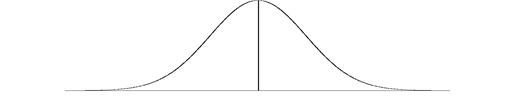
The readings or measured values of a quantity lie along the x-axis and the frequencies (number of occurrences) of the measured values lie along the y-axis. The Normal Curve is a smooth, continuous curve and is symmetrical about a central “x” value. The peak in frequency occurs at this central x value.
The basic idea here is that if we could make an infinite number of readings of a quantity and graph the frequencies of readings versus the readings themselves, random errors would produce as many readings above the “actual” or “true” value of the quantity as below the “true” value and the graph that we would end up with is the Normal Curve. The value that occurs at the centre of the Normal Curve, called the mean of the normal distribution, can then be taken as a very good estimate of the “true” value of a measured quantity.
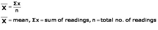
So, we can start to answer the question we asked above. The effect of random errors on a measurement of a quantity can be largely nullified by taking a large number of readings and finding their mean. The formula for the mean is, of course, as shown below:
Examine the set of micrometer readings we had for the diameter of the copper wire. Let us calculate their mean, the deviation of each reading from the mean and the squares of the deviations from the mean.
Поиск по сайту: